
by David Stainforth Tuesday, June 5, 2018
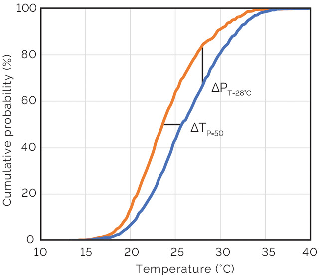
Figure 1. These cumulative distribution functions (CDF) represent the probability (P) of the maximum summer daytime temperature (T) around Bordeaux, France, being below a given temperature on the x-axis for the years 1950-1959 (orange) and 1993-2001 (blue). The separation between the two curves indicates a change in local climate between the two nine-year periods. For instance, median summer days (probability of 50 percent) warmed about 2 degrees Celsius (horizontal black bar), while the probability of the maximum temperature being below 28 degrees decreased from 83 to 66 percent (vertical black bar). Note that warmer days generally warmed more than cooler days (though the effect decreases for very hot days), indicating a change in the overall shape of the distribution rather than a consistent increase in temperature for all types of days. Credit: K. Cantner, AGI; data courtesy of David Stainforth.
Earth’s climate is changing. Increasing atmospheric greenhouse gas levels inevitably result in more heat being trapped in the lower atmosphere, the oceans and the land surface. But what does that mean where you are? What are the local consequences of global climate change? And what are the implications for decisions about how to adapt — decisions related to building design or flood protection measures, for example?
Most current efforts to understand and predict local consequences of global climate change use climate models. It is a challenge because local climates can respond in many ways to increasing global heat content, and such responses can vary considerably from one community to the next. Consequently, making reliable predictions about local climates places a high demand on the realism of computer models over a wide range of scales.
A complementary approach is to study historic changes using observational data. This is an approach that colleagues and I have pursued in recent years.
I don’t want to imply that observational analyses can provide predictions. Observations help us understand and assess models, but they also offer insights directly, potentially allowing us to make more robust decisions about adapting in the face of climate change.
The tricky part about using observational data to look at climatic trends is that we don’t observe or experience climate directly; we experience weather. You can think of climate as the distribution of potential weather conditions. Different conditions have different likelihoods of occurring, with closer-to-average conditions — average temperatures, winds or precipitation amounts, for example — usually more likely than outlying conditions. So, overall, climate can be represented by distribution curves that describe the probabilities of different conditions; these curves might be simple if portraying a single facet of climate, like temperature (see Figure 1), or they can be complex if representing multiple facets simultaneously.
Climate change alters the shapes of these distributions. For example, average daytime temperatures could increase. Or average nighttime temperatures could increase. Or both. The change could manifest as increased odds for extremely hot days and decreased odds of “typically” hot days, while the rest of the distribution stays pretty much the same. Each of these shifts would change the shape of a given climatic distribution in different ways, and changes to specific parts of a distribution are not necessarily related to a change in the average conditions. To understand if and how a local climate has changed, we need to quantify changes across the whole distribution, not just in the average.
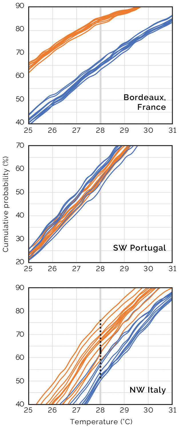
Figure 2. Comparing multiple pairs of CDFs offers a more robust picture of actual climatic change compared to any single CDF pair. Each curve again represents data from a nine-year period — orange and blue curves represent distributions from the 1950s-1960s and 1990s-2000s, respectively — and each pair is separated by 43 years, as in Figure 1. (Note that the x and y scaling is different relative to Figure 1.) Near Bordeaux (top), the climate at the 28-degree Celsius threshold has clearly changed. In southwestern Portugal (middle), the climate at this threshold has clearly not changed. In the Piedmont of northwestern Italy, there is no clear indication of the scale of any change because the smallest 43-year change is small (vertical solid black bar) while the largest change is large (vertical dashed black bar). Credit: K. Cantner, AGI; data courtesy of David Stainforth.
One difficulty in using weather observations to look for signs of local climate change is that the relatively short timescale over which recent, anthropogenic climate change has been occurring fundamentally restricts how well we can resolve changes.
To construct a climatic distribution from observations, we want to use as much data as possible so as not to be misled by sampling biases or outlier conditions. For instance, an unusually hot summer, if not averaged together with a sufficient number of other summers, can skew the overall shape of a distribution, such that the conditions portrayed by that distribution are not truly representative of longer-term climate. That means we must combine data from observations over multiple years.
In many locations we have daily weather observations dating back to the 1950s, and some processed datasets spatially interpolate these observations to provide time series of daily data gridded on a scale of roughly 50 kilometers — not quite “local” perhaps, but getting close. By using data from these time series — from 1950 to present day — we can extract the climatic distribution representative of that period for any available location. Or, we can extract distributions representing seasonal climates by only using data from certain months — say June, July and August if we want to look at the boreal summer climate.
If the climate weren’t changing, then such distributions would represent the climate today as accurately as they represent the climate in the ‘50s or anytime in between, and they’d be a good basis for making climate-sensitive decisions today. But we know that climate is changing globally, so we expect that local climates in most locations are also changing. Thus, we do not expect distributions built from data from the last 60-plus years to be representative of climate today. The challenge is to figure out how to use the available data to reveal how and where local climates are changing.
As a starting point, instead of using a whole 1950s-to-today dataset, we can compare portions of the data — say the nine years beginning in 1950 and the nine years beginning in 1993. Figure 1 shows distributions of daytime summer temperatures around Bordeaux, France, for those two time periods. The fact that the two curves do not overlap suggests that the climate near Bordeaux — at least with respect to the distribution of daytime summer temperatures — did change significantly in the latter half of the 20th century. In fact, the figure indicates that warmer temperatures were more likely across all types of summer days, from relatively cool days to average days to warm days.
Comparing two discrete time periods like this — rather than comparing single years — gives us a more accurate idea of how a local climate has changed. But it’s difficult to know just how accurate, in part because there is always the possibility that the sampled time periods still do not represent the underlying climate conditions because of natural variability. It would be nice to be able to compare conditions between two longer time spans — perhaps each 20 years long instead of nine, for example — but this is where the short overall timescale of recent global climate change bites us: the longer the time spans compared, the smaller the separation between them and the harder it is to identify signals of change.
One way to address this issue is to compare multiple pairs of distributions (Figure 2), with each pair separated by the same amount of time. In the example of Bordeaux, instead of just comparing two nine-year distributions beginning 43 years apart in 1950 and 1993, we can also compare the nine-year distributions beginning in 1951 and 1994, 1952 and 1995, and so on. Considering all these comparisons simultaneously shows us how much uncertainty there is among the distributions themselves, and gives us a more robust picture of the change that occurred compared to any single comparison between nine-year periods.
Unfortunately, the short duration of the last 60 to 70 years — the most interesting period to study with respect to climate change because it’s seen the fastest recent increases in global average temperature and atmospheric carbon dioxide concentrations — creates friction between clarifying signals of change, providing the essential context of natural variability, and resolving the distributions. That’s the challenge of observing local climate change.
So, what do the data reveal when we carry this exercise through? In Bordeaux (Figure 2, top), we see that the increase in daytime summer temperatures in the late 20th century was not only large but also robust — all the sample pairs reveal the same message. For example, the probability of the temperature exceeding 28 degrees Celsius — a threshold in some countries relevant for building design and management — rose from about 16 to about 35 percent. The results were different elsewhere, however. The same comparison for southwestern Portugal (Figure 2, middle) showed a small or nonexistent increase in the likelihood of days above 28 degrees, but the picture was again robust. In Northwest Italy (Figure 2, bottom), meanwhile, some pairs of distributions indicated a large change and others showed a small change, so the picture of climate change there is less clear because the variability in the distributions is itself large. (But at least we know that we don’t know, which is itself potentially useful.)
To support practical decision-making with respect to climate change adaptation on local scales, it’s helpful for researchers to focus on specific thresholds — like changes in the probability of days above 28 degree Celsius — and locations. But it is nevertheless interesting to look at patterns of change over larger regions.
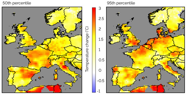
Figure 3. These plots show the smallest change in local summer daytime temperatures across 10 pairs of nine-year distributions (each pair is separated by 43 years) for average, 50th-percentile days (left), and for hot, 95th-percentile days (right). The character of climate change is different from place to place, but large-scale features can be seen. Identifiable warming of hot summer days, for example, is greatest in a band across Northern Europe, while for average summer days, warming is farther south, particularly in parts of France, Italy and Spain. The large changes indicated in North Africa are unreliable because the results are based on data from only a small number of observing stations. Credit: K. Cantner, AGI; data courtesy of David Stainforth from analysis of the E-OBS gridded datase.
Figure 3 summarizes changes in summer daytime temperatures across Europe using the same sort of analysis as described above — that is, comparing multiple pairs of nine-year distributions from the mid- and late 20th century. The figure shows local changes in two different thresholds: how much temperature has increased on an average (50th percentile) summer day; and how much it has increased on hot (95th percentile) days, for which only one in 20 days is hotter. In each grid square on the maps, what’s plotted is the smallest change seen from 10 pairs of distribution curves. This is a conservative approach: Where the change shown on the map is large (orange to red), we can be confident that there has actually been a significant change in summer daytime temperatures at that location (e.g., at least a roughly 2-degree increase on average summer days around Bordeaux in southwestern France). However, small changes on the map indicate either that there has been little change or that there is large variability in the differences between multiple pairs of distribution curves, so we can’t identify the change clearly with this method alone. Despite that shortcoming, the maps reveal interesting patterns in the changes in local climates. For example, hot summer days are clearly warming most in a band across Northern Europe, with increases of more than 2 degrees Celsius common, while warming of average summer days is centered farther south. The maps indicate significant warming at both thresholds in eastern Spain and eastern Italy.
This approach to using observational data focuses on identifying the character of changes in local climate over roughly the last 60 years. It reveals how these changes vary substantially from one place to another, even within relatively small areas. And it could be used to support decision-making that’s more robust and relevant to both today’s climates and those of the future.
In practice, many climate-relevant decisions are based not just on temperature but also on other variables. The approach described here has already been extended to identify changes in rainfall, including how much, or what fraction of, rain comes from events of particular intensities.
Changing climate can be experienced in very different ways in locations that may be quite close to one another. Although there are fundamental challenges to deciphering information about changing local climates from climatic distribution curves based on observational data, it is nevertheless often possible to extract useful, threshold-specific information. An important next step in this line of work is to focus on decision-specific vulnerabilities so that these data analysis methods can be used to improve the robustness and resilience of our societies.
© 2008-2021. All rights reserved. Any copying, redistribution or retransmission of any of the contents of this service without the expressed written permission of the American Geosciences Institute is expressly prohibited. Click here for all copyright requests.